Part IV- Shifts of IS and LM Curves

Synthesis of Monetary and Income Analysis - Part IV

Any fiscal policy change shifts the IS Curve, and any monetary policy change shifts the LM Curve.
a) Shift of the IS Curve due to changes in fiscal policy

The IS Curve shifts to the right to I'S' due to expansionary fiscal policy. Expansionary fiscal policy may be adopted through

i) Cut in taxes
ii) Increase in government expenditure
These are basically called real disturbances in the economy.

H becomes the new equilibrium position. When government spends more, there is an increase in income due to the operation of the multiplier. So the income increases to Yc from Ye. If national income increases, the demand for money also increases. This leads to an increase in the rate of interest, which now goes up to rc.

A cut or fall in taxes lead to an increase in the disposable income (Yd). Similarly this also leads to an increase in the rate of interest. Yd = Y - Tax.

The opposite thing will happen if the national income falls. The demand for money will fall. This would lead to a fall in the rate of interest.

b) Shift of the LM Curve due to changes in monetary policy

An increase in money supply or adoption of an expansionary monetary policy leads to a fall in the price of money, namely the rate of interest. This is basically called a monetary disturbance in the economy. Rate of Interest falls from re to rd. This shifts the LM Curve downward to L'M'. E' becomes the new equilibrium position. Due to a fall in the rate of interest, investment increases in the commodity market. Change in investment will increase the national income because ΔY = m(ΔI). National Income increases from Ye to Yd.

Thus, an increase in money supply leads to
a) Fall in the demand for money
b) Fall in the rate of interest
c) Rise in investment
d) Rise in the level of income

Similarly, a decrease in money supply leads to
a) Rise in the demand for money
b) Rise in the rate of interest
c) Fall in investment
d) Fall in the level of income

Any change in consumption function, investment function, government expenditure or taxes Shifts the IS Curve. Upward or downward shift depends upon whether the effect is expansionary or contractionary.

Any change in the demand for money, supply of money (or price level) Shifts the LM Curve. Again, upward or downward shift depends upon whether the effect is expansionary or contractionary.

c) There will be a number of possibilities if both the curves shift, due to simultaneous changes in monetary policy and fiscal policy.

If the IS Curve shifts to the right and the LM Curve to the left, the rate of interest increases from ro to r1, but income remains unchanged at Yo.
If both the curves shift to the right, the rate of interest remains unchanged at ro, but the level of income increases from Yo to Y1.
Various combinations of expansionary and contractionary monetary and fiscal policies may be adopted by the government to bring about the desired change in the economy.

Part IV of IV

Part III - Derivation of the LM-Curve and Equilibrium

Synthesis of Monetary and Income Analysis - Part III

Derivation of the LM-Curve and equilibrium

The derivation is based on the following three propositions.

1. An increase in the level of income leads to an increase in the demand for money.
2. An increase in the demand for money leads to an increase in the rate of interest.
3. Therefore, an increase in the level of income leads to an increase in the rate of interest.

The left part of the diagram shows the Demand for and Supply of money.
Ms is the supply curve for money.
Md is the demand curve for money.
E is the point of equilibrium in the money market.
Oro is the equilibrium rate of interest.
The right part of the diagram shows the relationship between level of income and the rate of interest in the money market, and the derivation of the LM_Curve.
OYo is the level of income.
Oro is the rate of interest.

Now income increases from Yo to Y1. So the demand for money will go up, and the demand curve for money, Md, will shift to the right. M'd becomes the new demand curve for money. F becomes the new equilibrium point, and the rate of interest goes up to Or1.

Now if we join the points E', F' etc. in diagram (b), we get the LM-Curve. 'L' stands for the demand for money (speculative) or liquidity preference and 'M' stands for the supply of money. The LM-Curve shows the alternative combinations of the rate of interest and the level of income for which money market is in equilibrium. In other words, at any point on the LM-Curve demand for money or liquidity preference is equal to the supply of Money.

General Equilibrium of the Commodity market and the Money market

We have shown two different equilibrium relationships between the rate of interest and the level of income, in the form of the IS-Curve and the LM-Curve. The commodity market and the money market are closely related to one another. Decisions regarding consumption and investment determine people's behaviour regarding wealth-holding between money and bond, and thus their demand for money. The rate of interest and the level of income in both the commodity market and the money market are the same.

Therefore the general (overall) equilibrium of the economy is ensured when the rate of interest and income are such that these are compatible with equilibrium in both the markets. The IS-Curve shows the equilibrium in the commodity market, and the LM-Curve shows the equilibrium in the money market. In other words, what it implies is that the values in question must lie on both the LM and the IS Curves for an overall equilibrium condition to be true. This can occur only when both the curves intersect.

Here both the IS and LM Curves are plotted on the same axes. The equilibrium level of income is given at Ye, where OYe is the equilibrium level of income, and that of interest at re, where Ore is the equilibrium rate of interest. Only at point G both the markets are at equilibrium. The diagram shows the general equilibrium of the commodity market and the money market. This is called the Synthesis of Monetary Analysis and Income Analysis, or the Synthesis of Fiscal Policy and Monetary Policy.

Part III of IV | Part IV: Shifts of IS and LM Curves

Part II - Derivation of the IS Curve

Synthesis of Monetary and Income Analysis - Part II

Derivation of the IS-Curve

The derivation is based on the following three propositions.

1. The rate of interest determines the level of investment (Autonomous). 2. The level of investment determines the level of income. 3. Therefore, the rate of interest determines the level of income.

Diagram (a) shows that lower the rate of interest, the higher the volume of investment.
Diagram (b) shows the relationship between income and investment.
We know that change in income = multiplier times change in autonomous investment
Or, ΔY = m(ΔI)
Or, m = ΔY/(ΔI)

If investment changes by a small amount, national income changes by a multiplied amount.

Corresponding to each level of investment there is a particular level of income. Here the rate of interest and the level of income move in opposite directions. Lower the rate of interest, higher is the level of investment and higher the level of national income.

The IS-Curve shows the alternative combinations of the rate of interest and the level of income, which bring about equilibrium in the commodity market. In other words, every point on the IS-Curve is a point of savings-investment equality.

Part II of IV | Part III: Derivation of the LM Curve and equilibrium

Synthesis of Monetary and Income Analysis - Part I

IS-LM Analysis - Commodity Market and Money Market Equilibrium

Macro Economics deals with the fundamental problems, which are concerned with determination of gross domestic output, income and employment, price level, and growth of national income. In the short-run determination of income, employment and price level are the primary concerns. Government policies, necessary to control these variables, are required to be ascertained, and put into use at the right time to accelerate or retard the economy.

Keynesian analysis is known as Income Analysis. The Monetary Analysis was done by classical economists. But this is actually a sysnthesis of Keynesian economics.

Economists Hicks and Hansen designed a model, which is popularly known as the Hicks-Hansen IS-LM Analysis. Assumptions of this analysis are as follows.

1. An economy consists of four types of markets, namely commodity market, money market, securities market and labour market.
2. There are enough resources available to produce the required quantity of goods and services, in accordance with the demand.
3. Any change in demand is reflected in a change in output.
4. Aggregate demand or expenditure consists of consumption expenditure, investment expenditure and government expenditure.
5. Aggregate supply consists of consumption goods and savings. To this we add tax collected (T), which is the income of the government.

I) Income Analysis - This is done in the commodity market. II) Monetary analysis - This is done in the money market.

Commodity market equilibrium condition
1. Consumption Function
'a' is the minimum level of consumption even at zero income. The income identity is Y = C + S (income = consumption + savings)
C = a + b*Y
Or, C = a + (ΔC / ΔY)*(Y)
Y = disposable income







2. Savings Function

s = ΔS / ΔY
3. Investment Function

Investment (I) = f(r), where 'r' is the rate of interest. Investment is inversely related to the rate of interest, as rate of interest is the cost of borrowing investment money.
This shows the equilibrium condition in the commodity market. The commodity market is said to be in equilibrium when the economy spends as much as it earns, or when income is equal to expenditure. That means when the supply side Y = the demand side E.
Y = E Or, C + S = C + I
C cancels out from both the sides of the equation, leaving S and I on either side, which are equal. That is, S = I (savings = investment)

Money Market Equilibrium condition

Demand function for money or Money-Demand function is Md = KPY + L(r)
where Md = demand for money
P = Price Level
Y = money income (gross national product)
PY = National Income or the money value of the goods and services produced. It is the real income.
K = proportion of money that is held for transactions purpose and precautionary purpose.
Transaction demand and precautionary demand depend upon the level of income. If the income increases, the demand for money also increases. Any increase or decrease in the rate of interest is unable to influence these two demands for money. Only speculative demand for money is influenced by the rate of interest.

"L" = Speculative demand for money or Liquidity Preference (that is, preference to keep liquid cash). 'L' is a function of the rate of interest. That is, L = f(r)
Suppose an individual is initially at point A. He is holding OMo amount of money, when the rate of interest is Oro. Money holding means the sacrifice of the current rate of interest. If the rate of interest goes up, an individual reduces his money holding, in order to earn the high rate of interest. Therefore, the rate of interest is called the opportunity cost of holding money, i.e. loss of the opportunity to earn interest at the current rate. Higher the rate of interest, higher is the opportunity cost of holding money, and consequently lower is the demand for money. People will then want to maintain their wealth in the form of bonds and securities.

Money Supply curve
Ms = C + D
C = currency in circulation in the form of notes and coins.
D = deposit or bank money
Money supply, Ms, remains fixed in the short-run, as it is controlled by the Central Bank, the central monetary authority. Equilibrium condition in the money market is established when Md = Ms (demand for money = supply of money).

Part I - of IV | Part II - Derivation of the IS Curve

Effects of Inflation

Effect on Production

During inflation producers try to minimize the risk. Hence a lot of production potential is sacrificed. Goods that are more durable are produced more; as compared to goods that are less durable. This alters the pattern of production.

Inflation gives rise to more speculation and hoarding, which is bad for the economy.

The basic knowledge about the market tends to lose its importance, and producers and consumers have to update themselves constantly.

Production and economic growth gets seriously retarded, as the products, at high prices, may fail to find a buyer.

Wrong anticipations and misallocation of resources lead to loss of profit and growth.

Effect on Distribution of Wealth

Inflation has its own effects on the aggregate demand, which in turn puts its effects on total production and income. Following are the several effects of inflation.

1. As demand for money increases, its price, namely the rate of interest, rises. That brings down the investment.

2. Inflation reduces the total output of the community.

3. As consumers feel insecure during periods of inflation, their desire to save increases. Thus, propensity to save rises.

4. As the value of money falls, and consequently the real value of wealth in the hands of consumers, spending made by the consumers fall.

5. As goods fetch higher prices in the domestic market, it discourages export, and to an extent encourages imports. More imports deplete the foreign exchange reserve of a country.

6. As profit expectation remains high due to high prices, it encourages investment in some way.

Redistribution of income and wealth take place during periods of inflation. Rate of growth of the economy in also reduced. During inflation people do not want to hold the money, whose value is falling. So there may be a conversion into other assets, in the form of bonds, securities or gold and silver. Wages and profits increase relatively more that rent and interest.

People belonging to the fixed income group are the major losers. Their earnings and accumulated savings diminish or get eroded. Debtors try to pay back their past debts in currencies which are of very little value.

Low-income groups suffer the most during inflation.

Effect on Employment

Inflation and unemployment are inter-related. A near full-employment situation with stability of prices is the aim. However measures to control inflation creates unemployment, whereas measures to reduce unemployment gives rise to inflation. It is like a trap. It is considered that a full-employment situation is a country's inflation threshold.

The Philips Curve merges the demand-pull and cost-push inflation and eliminates the distinction between them. It is proclaimed that the society itself chooses the best possible combination of price-level and employment. The least desired combination between the two could thus be eliminated by the society. Thus the Phillips Curve shows the trade-off between level of unemployment and wage-price increase. It is assumed that wage rise percentage is slightly more than price rise percentage. It shows that greater the unemployment, the lesser is the price rise, and vice versa. On the other hand, more the wage rise, less is the level of unemployment, and vice versa.

Social costs of involuntary unemployment are quite obvious. It cannot be ignored. Inflation can ultimately be considered as a severe form of taxation on the economy as a whole.'

Also read: Inflation and Deflation Demand-Pull Inflation Cost-Push Inflation

Cost-Push Inflation

Cost-push inflation is also known as Cost Inflation. It basically arises due to a rise in wage rates, which in modern economic conditions, are affected somewhat frequently due to pressure from labour unions. Interaction between demand for and supply of labour is no longer the only factor responsible for the determination of wage rates. That way we can say that wages rates these days are somewhat 'administered'.

Normally wage rate should increase only when there is excess demand for labour. Collective bargaining, through labour unions, is often responsible for a hike in wage rate, which has no relationship with the demand for labour exceeding supply. This way when the employers are forced to increase wages, their cost of production also increases. They cannot supply the finished goods at previous prices. Unable to curtail production, for which there may not be any apparent reason, producers and left only with the option of increasing the market price of the commodity.

It is very difficult to control this type of inflation through Fiscal and monetary policies. Through restrictive monetary and fiscal policies the aggregate demand can be brought down, which will bring down the price. But that affects economic growth, as production and investment gets curtailed and unemployment is created. Basically producers' profit is caught between restrictive monetary and fiscal policies on one side, and pressure for higher wages from labour unions on the other. Ultimately an understanding between employers and unions ascertain a stable wage rate that can drive out the inflationary price rise, where unions are faced with further unemployment, and producers are faced with reduced profits, both due to curtailed production.

Mixed Demand-Cost Inflation

Inflation may arise without an increase in general aggregate demand. Under a condition of full-employment, if there is an increase for a particular class of goods in the product or commodity market, it will push up the prices of that class of goods. This will induce producers to produce more of that particular class of goods. So more labourers or workers will be employed at a higher wage rate, as there is no idle labour force in the labour market. This may induce labourers in other industries to go for a wage hike as well, though there is no extra demand for labour in those industries. This way market prices of commodities will eventually go up due to increase in cost of production.

Also read: Inflation and Deflation Demand-Pull Inflation Effects of Inflation

Demand-pull Inflation

The classical theory states that inflation or constant price rise takes place when the quantity of money in circulation increases. The price rise is directly related to the percentage increase in the quantity of money.

Under a full-employment situation, when investment demand increases, there arises a total demand for goods, which outstrips the aggregate supply that is available. Prices then start going up. Consumer demand is dependent on disposable income. Sale of goods and services at higher prices creates more money income, and hence more demand. So the excess demand never gets checked.

Some price rise would occur even with a constant money supply. This price rise would increase the transaction demand for money, which will push up the interest rates. Higher interest rates would discourage extra investment demand. This would eliminate the inflationary effect.

We can explain demand-pull inflation with the help of inflationary gap. Inflationary gap may be defined as that part of government expenditure that is not covered by taxation or borrowing from the general public, and which is covered by borrowings from banks or other financial institutions, or by creation of money by the Government. Revenue spending of the Government then overruns revenue earning.

C+I+G shows the different expenditure levels at different levels of income. Equilibrium exists at point E, where the C+I+G cuts the income line. If, under a full-employment situation, the real income cannot reach Yo, but reaches only up to Yn, it gives rise to an inflationary gap, measured by XY.

If there is insufficient aggregate demand, there will be a fall in the C+I+G schedule. This is represented by the (C+I+G)' schedule. This will give rise to a deflationary gap, measured by YZ.

A boom in investment, technological advancements, opening up of new prospective territory etc. may give rise to some demand-pull inflation. However, increase in Government Expenditure, especially for the progress of backward areas, high defence expenditure etc. may also give rise to demand-pull inflation.

The inflationary gap may be eliminated in several ways.

1. Rate of interest can be increased by keeping the money supply constant. This will reduce investment, income and consumption. Prices will come down.

2. High prices will reduce the real value of wealth. This will reduce consumption expenditure and consequently prices. This is called the Pigou Effect.

3. If redistribution of income can be done in favour of the higher income group, consumption expenditure will come down. Higher income people will spend lesser portion of this redistributed income on consumption than the lower income group. The inflationary gap may come down in this way.

4. Extra tax collections will reduce the net disposable income. This will lower the consumption. Reduction in Government subsidies or welfare expenditure will also reduce disposable income and consumption.

5. Higher prices in the domestic market may discourage exports. This will increase supply in the domestic market. As a result, prices will come down. This may happen on its own.

Also read: Inflation and Deflation Cost-Push Inflation Effects of Inflation

Inflation and Deflation

Inflation may be defined as a rise in price level of all commodities in general. Effect of inflation on aggregate demand, and consequently on total production and income cannot be underestimated or ignored. A sustained trend of rising prices, or excessive growth of money income which surpasses the growth of real output, is the basic characteristic of inflation. Thus more money is required to buy the same quantity of a particular commodity. Real productivity fails to keep pace with price rise. The value of money keeps on falling.

Deflation is characterized by a falling tend in the general price level. This happens because of a fall in the aggregate demand. Deflation leads to increased unemployment, as there is a fall in investment due to a pessimistic behaviour on the part of investors. They invest less as the prospect of earning revenue is bleak. This causes unemployment and generates less income. Less income causes less demand.

Depression: If deflation comes at a time when there is sufficient unemployment in the economy, it is called Depression. It has a spiraling negative effect on the economy, and it becomes really difficult to boost it up.

Prof. Paul Samuelson has summarized inflation and deflation in the following words:

"By inflation we mean a time of generally rising prices for goods and factors of production - rising prices for bread, cars, haircuts, rising wages, rents, etc. By deflation we mean a time when most prices and costs are falling."

When money income in the hands of consumers increases, they acquire more purchasing power. The output of goods and services fail to keep pace with the purchasing power. More and more money runs after the same quantity of goods. This pushes up the demand, and consequently prices and costs of other factors of production. If production of consumer goods is cut down, then also there will be a situation of purchasing power, money income or effective demand outstripping actual supply. This will also push up the prices.

Once full-employment has been achieved, any increase in aggregate demand will push up the prices, leading to an inflationary situation. In such cases the economic infra-structure needs expansion. Additional production facilities, backed up by adequate investment, public (Govt.) or private, need to be generated to meet the rising demand.

Inflation may be of two basic types.

1. Demand-pull inflation: When effective demand overreaches actual supply, it is a case of demand-pull inflation. More money and fewer goods lead to a rise in prices.

2. Cost-push inflation: When costs of factors of production, like rent, wages and interest start rising spirally, it is a case of cost-push inflation. The cost of producing one unit of a commodity increases. This increases the market price of that commodity, which leads to inflation.

Stagnation: A period of no growth, or excessive slow growth of the economy, in terms of the gross domestic product, is termed as stagnation.

Stagflation: It is a situation where the economy is not growing, or growing at a negligible rate it terms of gross domestic product, but prices are increasing. It is characterized by persistent high inflation combined with high unemployment and stagnant demand.

An economic growth rate of 2%-3% or less is considered to be negligible.

Also read: Demand-Pull Inflation Cost-Push Inflation Effects of inflation

Role of Fiscal Policy and Monetary Policy

In reality there is always a gap between expectation and actual achievement. For a particular nation also this is true. There always remains a gap between actual GNP and potential GNP. (GNP = Gross National Product) The GNP that is produced in a particular year and the GNP that the economy is capable of producing, had there been high employment, optimum capacity utilization or maximum utilization of the available resources, are never equal. Even under favourable conditions, actual GNP falls short of the potential GNP. There is some wastage of scarce resources. Maintaining a steady growth with full employment and price stability is very difficult.

Fiscal Policy

When the economy does not function properly under the influence of unemployment, depression or inflation, the government tries to make certain changes in its expenditure policy to bring in the desired changes, and to eliminate the forces that are destabilizing the economy.

There are two basic measures that a government can undertake to stabilize the economy.

1. Government Expenditure

Increase in government expenditure acts as an investment. It gets added to the private investment that is prevailing in the economy. Thus, more government expenditure generates more employment and income, and takes the economy to a new equilibrium position.

C = consumption Expenditure
I = Private Investment Expenditure
G = Government expenditure
C+S+T = the income line of the community

FF is the full-employment line. It shows the society's maximum output capacity. The equilibrium is at point E. The society is not utilizing its full resources. This is known as under-employment equilibrium between investment and expenditure.

If the government tries to reach full-employment equilibrium, it will spend more money. As a consequence, the C+I+G curve will shift to a new position, C+I+G'. The full-employment level is reached at point F'. The government increases the expenditure by ΔG, and the national income increases by ΔY.

2. Taxation

Government Expenditure expands the economy, whereas taxation contracts the economy. More taxation reduces the disposable income of individuals. This reduces their capacity to spend on consumer goods. A rise in taxes lowers the C+I+G schedule or curve. This reduces income and employment. This is necessary during periods of inflation, when prices are moving upwards.

A reduction in taxes will give more income in the hands of consumers. Demand will increase, and new investment and income will be generated. This is necessary during periods of depression. Cut in taxes helps the economy to recover from a depressed state.

In a full-employment situation, increase in government expenditure will increase the income. But the economy cannot produce more to meet this extra demand, as it is already in a full-employment situation. Under such circumstances, prices will rise, leading to an inflationary situation. Then it is necessary to raise the taxes to take the extra income away, so that prices may not rise.

Similarly, lowering of government expenditure will lower the income, and effective demand. This may push the economy towards depression. So, with lowering of government expenditure, a reduction in taxes is necessary to maintain the same level of income and effective demand.

Monetary Policy

Monetary policy is aimed to control the supply of money in an economy. The central bank, which acts as the agent for the government, determines and controls the money supply according to the need of the economy. Objectives of monetary policy are as follows:

1. Price Stabilization
2. Move towards full-employment
3. Rapid growth rate
4. Stabilize the capital market
5. Favourable balance of payments.

Measures adopted to control money supply

1. Changes in cash reserve ratio
2. Changes in bank rate
3. Open market operations
4. Selective credit control
5. Moral persuasive measures

These two policies may be used in combination by the government to get the desired result.

Also read: Automatic Stabilizer and Discretionary Fiscal and Monetary Policy

Induced Investment and Thriftiness

In the topic Autonomous Investment and Thriftiness we have assumed that investment is independent of national income. That is not true. The investment schedule is not a straight line parallel to the X-axis. In reality entrepreneurs undertake more investment if sales and profit prospects improve. Thus they are induced to make more investments to satisfy the growing demand that influences the market. Even in the short run, the investment schedule takes the shape of a rising curve. More investment will generate more income and employment. Opportunities will increase, and producers will be induced to invest and produce more.

If we introduce induced investment with thriftiness the situations becomes worse than what it is with autonomous investment.

IpIp is the induced investment curve. It depends on the rate of change of GNP (Gross National Product). So the induced investment function is upward sloping. Ip stands for induced private investment. SS is the initial savings function, which cuts the induced investment function IpIp at E. An increase in thriftiness means an upward shift of the savings function SS to S'S'. F becomes the new equilibrium point. This corresponds to a lower level of income, OYf.
1. Aggregate savings goes up by ΔS.

2. As a result, national income falls by -ΔY.

3. Consequently, savings and investment will also fall from S = I to S' = I'.

An increased desire to save leads to a fall in savings due to a fall in income.

The Paradox of Thrift

Thus the policy of thriftiness is self-defeating. People want to save more but due to a fall in income, the savings also comes down. An increase in thriftiness leads to a fall in income, since the multiplier process acts in the negative direction. This leads to a fall in savings. So the society, at the end, saves less, not more.

Must also read: Autonomous Investment and Thriftiness

Autonomous Investment and Thriftiness

Thriftiness

Thriftiness means an increased desire to save or a decreased desire to consume. In other words, it implies an upward shift of the savings function, or what comes to the same thing as a downward shift of the consumption function. b↓ + s↑ = 1, where b = Marginal Propensity to Consume, and s = Marginal Propensity to Save.

The classical economists argue that thriftiness is beneficial for the society. This is because more savings means more capital formation, and more output of consumption and capital goods.

This view was challenged by Mr. J. M. Keynes and he said that if the economy is in depression, the problem is one of raising the effective demand. Under this situation, an increase in thriftiness means a fall in demand and ultimately a fall in income through the multiplier.

Autonomous investment and Thriftiness

Autonomous investment is completely elastic, as it has no relationship with Gross National Product (GNP) or its rate of change. Level of autonomous investment depends upon rate of interest and marginal efficiency of capital.

SS is the original Savings function where OYe is the National Income. II' is the Investment Function. Aggregate Savings S = s(Y), where s = MPS or marginal Propensity to Save. E is the equilibrium point where savings = investment. When savings is equal to investment, national income is equal to national expenditure. Therefore, OYe is the equilibrium level of income.

If there is an increase in thriftiness or an increased desire to save, the savings function will move upwards to S'S'. Then EF measures the increase in savings (ΔS) at the same level of income. Income remains the same but savings increases, resulting into a reduction in consumption. Now the new Savings Function, S'S', cuts the Investment function II' at G. So G is the new equilibrium point and it corresponds to a lower equilibrium level of income, OYg. Therefore national income falls by ΔY, due to an increase in savings by ΔS.

So savings is damaging to the economy. Ultimately, it lowers the income.

Must also read: Induced Investment and Thriftiness

Purpose Of Keeping Accounts

Generally people have a short memory, and businessmen are no exceptions. They have to do many transactions daily. A businessman gives cash to and receives cash from a number of suppliers and customers. He purchases and sells goods and other articles for cash and on credit. He incurs a number of expenses daily and earns income from different sources. At times he sells business properties, which are no longer required, and at other times makes additions to properties already existing. He cannot remember for long all the varied transactions taking place daily in his business. He must, therefore, make a written record of his varying transactions, so that in times of need he may refresh or supplement his memory by referring to his written records. In other words, he should keep accounts.

Book Keeping is the art of recording daily business transactions regularly in a set of books, following a definite system.

- Only the transactions of a financial nature are recorded.
- The recording of transactions is made in a definite set of books specially designed for the purpose.
- Records are maintained date-wise.

Accounting: Accounting is preparation of statements or accounts in a summarized and classified manner to find out the profit or loss, and to ascertain the financial position of the business. Accounts are maintained in a "T" form.

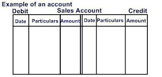
Meaning of DEBIT and CREDIT: The left hand side of each account (utilized for recording transactions in respect of which that account has received benefit) is called the "debit" side, and the recording of transactions on the debit side of any account is technically known as "debiting an account". Thus, to debit an account means to enter the transaction on the debit (left) side of that account.

Similarly, the right hand side of each account (utilized for recording transactions in respect of which that account has given benefit) is called the "credit" side, and the recording of transactions on the credit side of any account is technically known as "crediting an account". Thus, to credit an account means to enter the transaction on the credit (right) side of that account.

Double Entry System of Book Keeping: Every business transaction has a two-fold effect. It affects two different accounts in opposite directions. A complete record of any transaction would, therefore, require the entry to be made in both the accounts, debiting the one and crediting the other. This recording of the two-fold effect of every transaction is known as Double Entry. According to William Pickles, the two-fold effect of every transaction is recorded under double entry system - one effect being the receiving of some benefit, and the other being the giving of some benefit. In other words, every transaction involves two accounts, a receiving account and a giving account. The receiving account is debited and the giving account is credited.

Trial Balance: At the end of  the financial period, which is normally a year, (may be less) if the debit and credit sides of every ledger account is totalled and all accounts' individual balancing figures, either debit balance (debit side heavier) or credit balance (credit side heavier) are taken into consideration and columned up into two debit and credit columns, their totals should tally, since every debit has a corresponding credit under double entry system of book keeping.. This statement is called trial balance. A trial balance should always tally (total of debit balances = total of credit balances) irrespective of when it is prepared.

Manufacturing account and trading account: A manufacturing concern needs to prepare a manufacturing account as well as a trading account. A trading account is required to be prepared by all.

In the manufacturing account (in the same "T" form) all manufacturing expenses' balance from the trial balance are written. This total gives the total manufacturing cost.
All expenses always have a debit balance. So these manufacturing expense accounts in the ledger are closed
by transferring them to the manufacturing account thus:

Respective Expense account
 - credit side: By manufacturing account      say 20,000
Manufacturing account 
- debit side: To respective expense account           same 20,000  (double entry completed, and the respective expense account gets closed, with no balance)
Total of all manufacturing expense balances thus get transferred to the manufacturing account. Now the manufacturing account has all debits which gives a total, say 5,00,000. Then the manufacturing account is closed by transferring this debit balance total of 5,00,000 to the trading account in the folowing manner.

Manufacturing account
 - credit side: By Trading account   5.00,000

In the trading account the manufacturing cost (as ascertained from the manufacturing account) is tranferred by completing the double entry thus:
In trading account 
- debit side: To manufacturing account   5,00,000. Just balances get rolled over from one account to the other.
If it is not a manufacturing concern, then there will be no Manufacturing Account, but only Trading Account.
Then,
In trading account 
- debit side: To Purchases account   5,00,000.  (from trial balance, Purchases account debit balance)
Now other "direct" trading expenses (wages, carriage inward etc), again from the trial balance, are posted in the Trading accont thus. (the same way as all the manufacturing expenses are posted in the manufacturing account above.)

In trading account 
- debit side: To respective expense account balance from trial balance  say, 10,000 (there may be multiple trading expenses. Same treatment for each.)

Trading account Total now comes to say 5,00,000 + 10,000 + 5,000 + 25,000 = 5,40,000

In the credit side of the trading account we write: By sales account  say 7,50,000 (this 7,50,000 sales account credit balance figure again comes from the trial balance)

The balancing figure 7,50,000 - 5,40,000 = 2,10,000 is the gross profit earned. Had sales been less than 5,40,000 (say 5,00,000) it would have resulted in a gross loss to that extent (40,000).

Again rolling this gross profit or gross loss to the next account, namely Profit and Loss Account, takes place thus:

In Trading Account 
Credit side
- By Profit and Loss account  2,10,000 (gross profit transferred to P/L account)
or
Debit side
To Profit and Loss account  40,000 (gross loss transferred to P/L account)

Profit and Loss Account: Remaining indirect expenses' and indirect incomes' account balances, again from the trial balance, are transferred in the same way in the Profit and Loss account.

Profit and Loss Account
-----------------------------------------------------------------------
To Trading account  (gross loss)     40,000    OR  By Trading account (gross profit) 2,10,000 
To other respective indirect expense    2,000               By other respective indirect income 500
---- more -----                                                   --- more ----

Balancing figure gives net profit or net loss which is either debited (if loss) or credited (if profit) to the Capital Account.
----------------------------------------------------
                                 Balance Sheet
Liabilities                            |                     Assets

Now in the trial balance, the balances that remain unused are all either assets or liabilities. Those are put here. Total assets (machinery, furniture, cash/bank, money receivable etc) must always be equal to total liabilities (internal:  liability of the business towards the owner, that is the capital contributed by them(shares etc), AND external: towards outsiders, like money payable)

Total assets must always be equal to total liabilities.

This finishes the Final Accounts part, where somewhere or other every ledger account balance, either debit or credit, as shown in the trial balance, must necessarily have been used.

The owner now know the profit or loss, as shown in the Profit and loss Account, and the financial position of the company, as shown by the Balance Sheet.

Hierarchy of preparation: Trial balance, Manufacturing account, Trading Account, Profit and Loss Account and Balance Sheet.
-------------------------------------------
Golden rule of accountancy

There are basically three types of accounts
1. Personal account:
                      Debit    : the receiver of benefit
                      Credit   : the giver of benefit

2. Nominal  account: ( All expenses and incomes)
                      Debit : All expenses and losses
                     Credit : All incomes and gains

3. Real Account: All assets and liabilities
                      Debit: what comes in
                      Credit: What goes out.
--------------------------------------------------------------------
Trial Balance is prepared on a particular date.

Manufacturing, Trading and Profit and Loss Accounts are prepared for a particular period.
                    say, for the year ended March 31, 2014

Again, Balance Sheet, showing the financial position of the company, is always "as on a particular date."

Up to maintenance of ledger accounts, that is journal entry, double entry ledger posting, it is book keeping.
Preparation of Trial Balance, Manufacturing, Trading, Profit and Loss account and balance sheet is accounting. Accounting starts where book keeping ends.

------------------------------------------------------------------------
Simply, every account is like a tank. One side dumping/recording the "in(s)" and the other dumping/recording the "out(s)", and then finding the balancing figures and working with those balancing figures, starting from preparation of Trial Balance.

Simple Income Determination with Savings-Investment Equality

National income is the sum total of consumption and savings. It is the money value of all commodities and services produced in the economy. These commodities and services are of two types.

1. Supply of consumption goods and services

2. Supply of Capital (investment) goods and services.

'Y' is the aggregate supply because it is the sum total of consumption and savings. Y = C + S. To this we add tax collected (T), which is the income of the government. Then the equation becomes Y = C + S + T.

Expenditure 'E' means aggregate demand. It is composed of aggregate consumption expenditure, or demand for consumption goods and services, as well as aggregate investment expenditure, or demand for investment goods and services.
Thus E = C + I. To this if we add government expenditure (G), then the equation becomes E = C + I + G.

We know that at equilibrium, income is equal to the expenditure for the economy as a whole.

In the whole model, where there are three sectors, the consumers, the business firms and the government,

1. Income = consumption + savings + Tax. Y = C + S + T - This is the supply side.

2. Expenditure = consumption Expenditure + private Investment Expenditure + Government Expenditure - E = C + I + G. This is the demand side.

If Y = E, then C + S + T = C + I + G

In an equilibrium position, government income, in the form of tax, is equal to government expenditure. T = G.

C + S + T = C + I + G. 'C' cancels out from both the sides, and T = G. Then, as because income 'Y' is equal to expenditure 'E', savings = investment, or S = I. This is known as the equilibrium condition of the national income. This can be shown with the help of the following diagram.

We initially draw a 45 degree line OY where Y = C + S + T. This is the income line of the community. At any point on this line, income = expenditure, or every point is a point of national income equilibrium. I-I' is the fixed level of autonomous investment, irrespective of the level of national income.

Now if we merge the Y = C + S + T supply (income) schedule, the 45 degree line, and the demand (expenditure) schedule E = C + I + G, we can arrive at the equilibrium position.

The savings curve is upward sloping, because with every increase in income, savings increases. Refer to the Savings function in earlier posts.

E is the equilibrium point.

At point F, aggregate demand is greater than aggregate supply. So prices will go up. More goods will have to be produced in order to meet the excess demand.

FF' measures excess of expenditure over income. This is known as the Inflationary Gap. It shows that the community is attempting to consume more than what it is capable of producing. Due to this excess demand, prices will go up, and further production will be profitable. If production increases, National Income will also increase, until the equilibrium level of income is reached.

At point G, income is greater than expenditure, and GH measures what is called Deflationary Gap. The community is consuming less than what it is capable of producing, or demand is less than the supply. Producers are now faced with the problem of unintended accumulation of inventories. As a result prices will fall, and production will also fall, until the inventories are run down completely. In the process it will come back to the equilibrium point E. At the equilibrium point prices will be stable, because there will be neither inflation nor deflation.

Induced Investment and the Accelerator

The proportion of Gross National Product (GNP) that enters into investment goes a long way to determine the economic growth of a country. Autonomous investment is determined by rate of interest and marginal efficiency of capital. It does not change with the change in national income. However, the other type of investment, namely Induced Investment, varies with the national income. With every increase in National Income, induced investment keeps on increasing. It is called 'Induced' because a change in National Income induces a change in investment.

Example: National Income changes from $1,000 billion to $2,000 billion, and induced investment changes from $200 billion to $400 billion

Change in National Income = ΔY = $1,000 billion

Change in induced investment = ΔI = $200 billion

Then, Marginal Propensity to Invest (i) = ΔI/ΔY = 200/1000 = 1/5

Change in Induced Investment divided by change in National Income gives us the Marginal Propensity to invest, denoted by 'i'.

Example:
The accelerator shows the accelerated effect on investment due to a small change in output or sales. 'v' is the accelerator or capital/output ratio. It shows the amount of capital required to produce one unit of output.

When output increases by 25 units, from 75 to 100, and the value of 'v' is 2, capital stock must increase by 50 units. This increase in capital stock is nothing but investment.

Thus, induced investment depends on the rate of change of GNP and the accelerator. If sales or output fails to increase period after period, no new investment will be undertaken. Therefore, for net investment to be positive, it is essential that output must not only be high; it should be changing. This is the Acceleration Principle.

The Accelerator illustrated
Net investment = change in capital (requirement) stock

We assume that there is a constant rate of depreciation of $10 per unit. Gross investment is net investment + depreciation.
A small change in output will lead to an accelerated change in investment. When output increases by 20%, gross investment increases by 200%. For every 1% increase in output, there is a 10% increase in gross investment.

When output fails to increase in the 6th year, gross investment drops down by 75%.

If output starts falling, net investment will be negative, and the firm will start selling some of its capital equipments. Gross investment will take place to the extent of depreciation only.

The accelerator is a very powerful factor and it works with the multiplier in causing cyclical fluctuations in business activities.

Autonomous Investment

Autonomous investment is that investment which is independent of the national income. It takes place on its own, without bearing any relationship to Gross National Product or its rate of change. If we analyze the factors that govern autonomous investment, then we will clearly understand why it is autonomous. Autonomous investment depends upon two major factors.

1. Rate of Interest 2. Marginal Efficiency of Capital

1. Rate of Interest: Rate of interest is the cost of borrowing money in order to acquire an asset, or if funds are available, then the income or opportunity, in the form of interest, foregone to acquire the asset. The later is called the opportunity cost of investment.
Investment is inversely related to rate of interest. The higher the rate of Interest, the lower will be the level of autonomous investment. A fall in the rate of interest will bring in fresh investment. Fresh investment will increase income through the multiplier, and employment will consequently rise.

2. Marginal Efficiency of Capital: It is basically concerned with the rate of return from the investment. Investor's expectation from future earnings from the investment must always be greater that the cost of borrowing the necessary funds, required to acquire the asset. This expectation is largely dependent on present level of expenditure and consumption. If these are high, then the investor will have an optimistic view of the future. He will invest.

So long as the present value of future earnings from the asset is equal or greater than the acquisition cost of the asset, the producer will invest. Marginal efficiency is basically a rate, at which future yields, expected from one additional unit of an asset, must be discounted, so as to make the total yield at least equal to the acquisition cost of the asset.
Marginal efficiency of capital, within a given period of time, keeps on diminishing for any given kind of asset. This is because anticipated yields from the asset will diminish, as more and more of the asset in put into use. Secondly, the acquisition cost of the asset will increase as more and more of that asset is purchased by producers.

The concept of autonomous investment was developed by Mr. Keynes. He said that autonomous investment would be positive, so long as the marginal efficiency of capital is greater than the rate of interest. So long as mec > i, fresh investment will take place. If the market rate of interest remains unchanged at oi, and the marginal efficiency of capital starts falling with the application of more and more capital, a stage will be reached when when mec = i. This is shown by the point E, where the producer will reach his optimum level of investment. This occurs due to the Law of Variable Proportions.

Investment - An Overview

Investment Function

National income is denoted by Y. It has two components, consumption(C) and savings(S). A part of the income is spent on consumption. That which is not spent is obviously saved. It may or may not be invested.

So we can say that Y = C + S

C is the supply of consumption goods and S is the supply of savings. This is the supply side of the picture.
National income is basically the money value of all goods and services produced in an economy during an accounting year. Total goods produced or total production is the sum total of consumption goods and capital goods. The total expenditure of the community is denoted by E. It means aggregate expenditure or effective demand. Aggregate expenditure is called effective demand because whatever is spent must be backed up by an equivalent demand.

So we can also say that E = C + I

C is the demand for consumption goods, or expenditure made by the household sector. I is the demand for investment made by the private firms. This is the Demand side of the picture.

National Income is said to be in equilibrium when the country spends as much as it earns, or when income is equal to expenditure. That means when the supply side Y = the demand side E.

Y = E Or, C + S = C + I

C cancels out from both the sides of the equation, leaving S and I on either side, which are equal.

That is, S = I. So the major point is that Savings (S) is equal to investment (I), only when the national income is equal to national expenditure. Gross national income is the money value of Gross National Products (GNP).

Investment is the second broad component of GNP. Although savings = investment, there is a relationship between savings and investment. Savers save more when the rate of interest is high, and investors invest more when the rate of interest is low. Although savings is equal to investment, savings is positively related to rate of interest, and investment is negatively related to it.
Definition: Investment refers to the change in the stock of capital either of the economy or of a business firm between two periods.

Dual Aspects of Investment: Investment is a form of expenditure and a source of demand. We know that E = C + I. Investment also shows the change is the stock of supply of capital. By adding to society's stock of capital, we enable it to produce more of both consumption goods and capital goods in future.

Gross Investment and Net Investment

Here D means depreciation. Gross investment less depreciation provides us with net investment or net capital formation.
Depreciation is defined as the reduction or depletion in the value of an equipment due to its contribution to the production process. It includes normal wear and tear.

Multiplier Theory of J. M. Keynes

We know that there are two key concepts Marginal Propensity to consume (MPC), and Marginal Propensity to Save (MPS). What is not consumed is automatically saved, and what is saved, a part or whole of it is automatically invested. The savings in done by the consuming, household sector, and the investment is done by the producing sector.

Change in Income(ΔY) = $100
Change in Consumption(Δ) = $80,
Change in Savings(ΔS) = $20
We also know that ΔY = ΔC + ΔS
Dividing both sides by ΔY,
We get ΔY/ ΔY = ΔC/ΔY + ΔS/ΔY
Or, 1 = ΔC/ΔY + ΔS/ΔY
Or, 1 = 80/100 + 20/100
Or, 4/5 + 1/5 = 1
Or, b + s = 1

We can now use an imaginary table.

Prof. Keynes introduced two major inferences.

1. If income increases, consumption will also increase, but less than proportionately (as part of the change in income is saved.)

2. The Marginal Propensity to Consume (MPC) is less than Average Propensity to Consume (APC). Average Propensity to Consume is Total Consumption divided by Total Income.

The Multiplier

b + s = 1
Or, s = 1 - b
Or, 1/s = 1/(1-b) = the multiplier "m".
"m" is the reciprocal of the marginal Propensity to Save.
m = 1/s = 1/(ΔS/ΔY) = 1/{1-(ΔC/ΔY)}

According to Mr. Keynes, the change in income ΔY = multiplier times change in investment, ΔI.

According to our above example, b = 4/5 and s = 1/5

Therefore, m = 1/s = 1/(1/5) = 5

ΔY = m(ΔI)

If investment changes by $100, then income changes by

ΔY = 5($100) = $500

Thus if investment increases, national income will also increase, not by the same amount, but by a multiple of it. Another point made by Prof. Keynes was that if the consumption expenditure of the community increases, the value of "b" will be larger and larger, and so also the value of the multiplier, and so also the national income.


The multiplier is the reciprocal of Marginal Propensity to Save. Corresponding to each value of "b" there will be a particular value of "s", and corresponding to each value of "s", there will be a particular value of "m".
Change in income ΔY = multiplier (m) times change in investment, ΔI

The Logic of the Multiplier
According to Mr. Keynes, the multiplier means that a small increase in investment will lead to a multiple increase in income. One man's expenditure is another man's income, and vice versa. When a man spends a part of his income, say $X, he creates an income of others of $X. The second person will again save a part of $X, and spend the rest. Again, the second man's expenditure creates an income for the third person. Thus the same money goes on creating incomes for a number of persons. This process leads to the following equations, where "b" is the part of the income spent, or MPC.


Larger the value of "b", greater will be the change in income.
The root cause of unemployment is deficiency in demand. And the only way to stimulate the economy in depression is to increase the demand through public or government expenditure programmes. Fresh expenditure will generate new incomes, and the multiplier process will set in. The multiplier effect will ultimately restore the full-employment situation.

Assumptions: In order to explain the Multiplier theory Mr. Keynes made the following assumptions:

1. Consumption always changes with change in income. In other words, consumption will always depend on income.

2. Marginal Propensity to Consume will remain constant.

3. There is change in Autonomous Investment. Autonomous Investment means when investment takes place even when there is no increase in income.

Limitations: The following factors will set a limit to the working of the multiplier.

1. Leakages: The higher the Marginal Propensity to Consume, the higher will be the value of the multiplier. The income, which is received, should be spent, so that it may again come back as income. If people prefer to keep cash balances idle, for transactions, precautionary or speculative motives, income created will naturally be less.

2. Consumption Goods: With the rise in income, consumption goods should be readily available in sufficient quantities, so that additional income may be spent on them. If there is shortage of goods, additional income received may not be fully spent. The Marginal Propensity to Consume will be low, and therefore the multiplier will be low.

3. Multiplier Period: The time gap between the receipt of income and consumption expenditure is known as the Multiplier Period. The smaller the time span of the multiplier period, the higher will be the value of the multiplier.

4. Investment: Any increase in investment in one sector should not be accompanied by a decrease in investment in another sector. Increments in investments should be repeated at regular intervals.

5. Full Employment Ceiling: If the economy is working at or near full-employment level, fresh investment outlay cannot lead to an increase in the supply of consumption goods. It will not raise aggregate income but will lead to price rise. Full-employment situation is called the economy's inflation threshold.

6. Induced Investment: Just as a change in investment induces consumption, so also induced consumption can influence investment. But the multiplier effect does not take this into consideration.

Conclusion: Though there are some limits in the workings of the multiplier, Mr. Keynes used this concept to advocate public investment during a period of depression.


Must also read: 1. Consumption and savings
2. Consumption Function and Savings Function

Consumption Function and Savings Function

Before reading this, read: Consumption and Savings

1. Consumption Function
The income identity is Y = C + S (income = consumption + savings)

C = a + b*Y Or, C = a + (ΔC / ΔY)*Y

MPC or Marginal propensity to Consume is "b". Y is the total income and b = ΔC / ΔY
In the diagram, "a" is the minimum consumption necessary to maintain oneself even at zero income. Now suppose the income increases to B. So AC is our familiar ΔY (change in income). Income increases from O to Yo, which is equal to AC. BC measures change in consumption ΔC, which is the resultant increase in consumption due to an increase in income.


2. Savings Function

MPS or Marginal Propensity to Save is "s". Y is the total income and s = ΔS / ΔY

Income multiplied by Marginal Propensity to Save or MPS or "S" will give us the total savings of the community.

Any point below the point B shows negative savings. B is called the break-even point or the point of zero savings. This means at point B, income = consumption and MPC = 1, as because MPS = 0.

The economic rationale is that at low levels of income people consume more than they earn. At a certain minimum level of income, income is exactly equal to consumption. This is the break-even point in consumption, where savings = 0. Thereafter, with every increase in income, savings goes on increasing. Therefore MPS or s = change in savings / change in income = ΔS / ΔY.